Prolly Trees are the magical data structure that makes the Dolt family of version-controlled databases possible. I wrote the canonical opus on Prolly Trees a little over two years ago. I thought that documentation would never be topped, but I’m pretty sure I’ve outdone myself today.

Can I interest you in an interactive Prolly Tree visualizer powered by DoltLite that runs entirely in your browser via WebAssembly (WASM)? I’m so proud of my new creation that I’m the proud new owner of prollytree.com, which hosts the new visualizer.

Powered By DoltLite#

I’ve been looking for a great DoltLite demo. DoltLite is embedded, like SQLite, so it can run in a browser. We package a WASM build on npm as @dolthub/doltlite-wasm. The approximately 3.4MB module downloads on first load, and everything after that happens locally. No database server. No rows sent over the network.

The visualizer does not fake a Prolly Tree in JavaScript. Every insert, update, and delete is SQL executed against DoltLite. After each operation, the visualizer streams the open database out of DoltLite’s virtual file system, reads the DoltLite v12 chunk store, finds the table root in the catalog, decodes the actual Prolly Tree nodes, and draws them as SVG.

The public SQL interface handles all table creation, mutations, row reads, and the dolt_hashof_catalog() call that identifies the current working catalog. SQL does not expose the physical tree. The WASM export sqlite3__wasm_db_export_chunked() streams the database bytes out of DoltLite’s virtual file system, and the visualizer’s TypeScript decoder reads the on-disk chunk and Prolly Tree formats to recover chunk boundaries, levels, sizes, and child addresses.

Here is the full path:

browser control
  → SQL against DoltLite WASM
  → DoltLite's C Prolly Tree engine
  → DoltLite v12 database image
  → real node bytes and child hashes
  → SVG visualization

The keys, chunk sizes, tree levels, and 40-character content addresses you see on screen all come from the real stored bytes. You can click a node to inspect its full address, encoded size, keys, SQL values, or child addresses. No simulated trees allowed.

Created By Codex#

The visualizer is also another win for agentic development. Oh my God, this would have taken me a year to muck with this much React and CSS. Like low-level C in DoltLite itself, my React and CSS skills are basic. I cannot make a tree animated and look good on a 13-inch laptop. Codex apparently can.

Codex is now incredible at this type of project. The storage format, the tests, and DoltLite itself provided a hard specification. I supplied the product direction: make the Prolly Tree opus interactive, use the real engine, and make every important property visible. Codex supplied the TypeScript, SVG layout, animation, tooltips, tests, and seemingly endless CSS. This all took about eight hours of back-and-forth from start to finish. The result feels like a real application, not a data-structure toy. Want to see how it works? The source is on GitHub.

The Tour#

The goal was to show off the four primary attributes of a Prolly Tree:

1. B-tree-like performance on reads and writes
2. Fast diff
3. Structural sharing
4. History independence

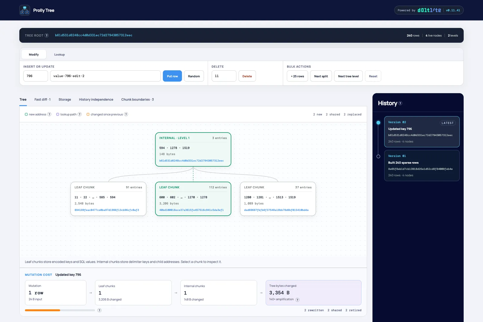
The visualizer starts with 240 sparse integer-keyed rows. That is enough to produce a two-level tree with one internal node and three leaf chunks. Each node displays its key range, encoded size, and content address. The timeline on the right (or bottom if you don’t have a wide screen) keeps every state created during the session so you can move backward and forward through the tree.

Now, let’s break it.

Modify#

A Prolly Tree is immutable. To update a row, you seek through the internal nodes to the leaf containing the key, copy and edit that leaf, calculate its new content address, and then rehash every internal node on the path back to the root. Unchanged chunks keep their old addresses and are shared with the previous tree.

Insert and delete work the same way, with one extra wrinkle: changing the keys can create or remove a content-defined chunk boundary. If the boundaries do not change, you still only rewrite one path from leaf to root.

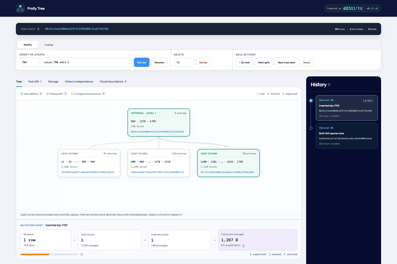
Here I randomly inserted key 1755. The rightmost leaf and the root turned green because they have new content addresses. The other two leaves are unchanged and shared. The mutation-cost panel makes the write amplification explicit: a 19-byte row produced 1,267 bytes of new tree data, but only two of the four live nodes were rewritten.

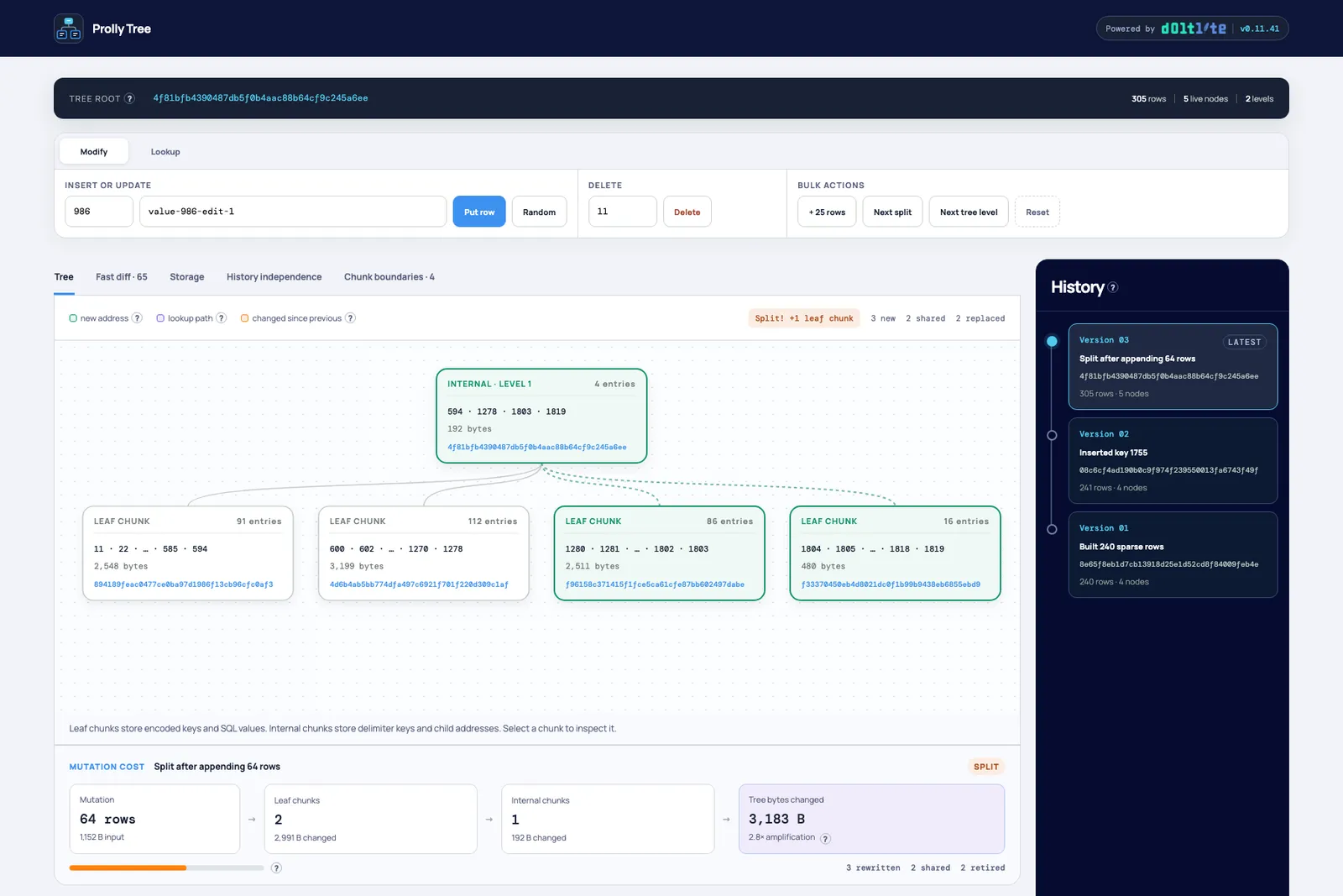
You can insert or update a specific key, delete a key, make a random edit, or append 25 sequential rows. The Next split button keeps inserting until the number of leaf chunks increases. In this run, 64 appended rows created one new leaf. Three chunks were written while two existing leaves remained shared.

There is also a Next tree level button. It inserts rows with wide values so you can grow a three-level tree without clicking for the rest of your natural life. The browser demo stops at three levels because it renders every node in full. A fourth level can fan out to hundreds of thousands of leaves. That is great for a database and terrible for a browser canvas.

Lookup#

Point and range lookups work like B-tree lookups. Internal nodes contain delimiter keys and child addresses. For a point lookup, start at the root, choose the child whose range can contain the key, and repeat until you reach a leaf. That is O(log n). A range lookup pays O(log n) to seek to the start and then reads the matching leaves, for O(log n + k) total work.

The visualizer animates the route in purple. Looking up key 796 in this tree visits the one internal node and one of the three leaf chunks. The other two leaves are never read.

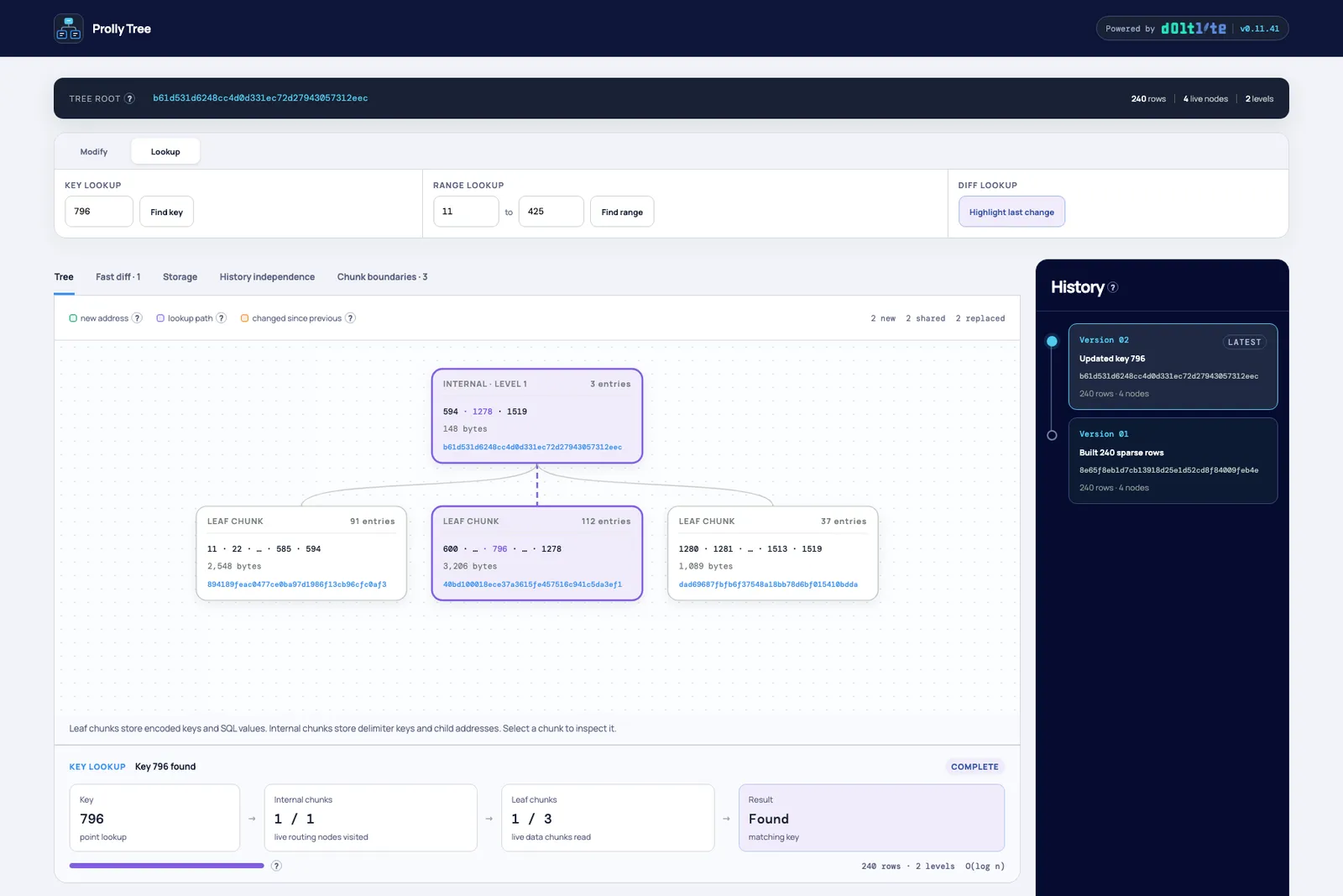
The Highlight last change button performs a different kind of lookup. It compares the current tree with the immediately previous tree. Orange chunks have different addresses and must be opened. Dashed chunks have matching addresses and represent whole subtrees that can be skipped.

In this example, updating one row requires four address comparisons and opening two changed chunks. Two shared subtrees are skipped, avoiding inspection of 128 rows. The diff lands on the changed leaf and emits one row difference.

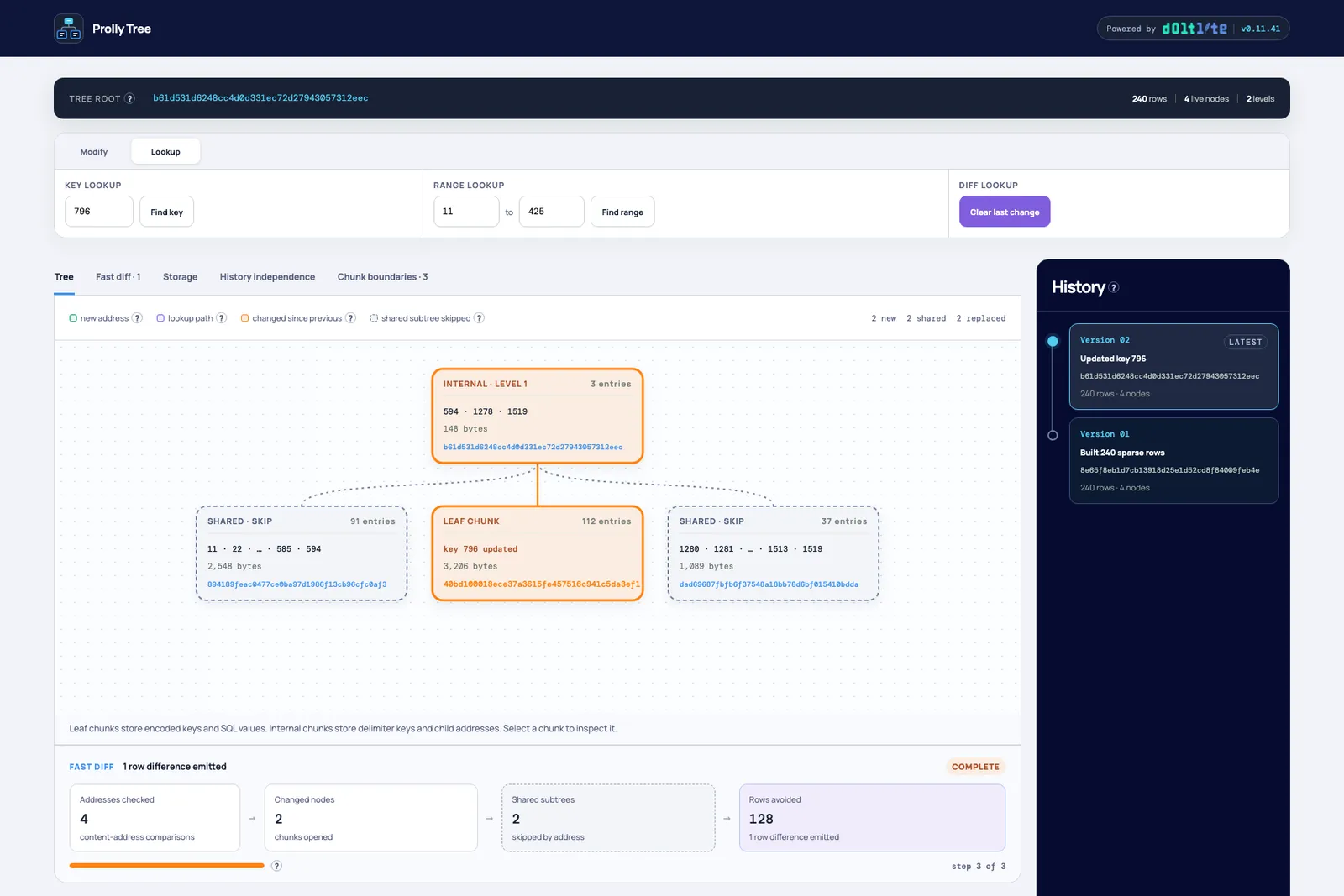
That is the bridge from ordinary B-tree-style lookup to one of the Prolly Tree superpowers: fast diff.

Fast Diff#

The Fast diff tab compares the current tree with any earlier version in the timeline. The algorithm starts by comparing root addresses. If they match, that means the trees are identical, and the diff is done. If they differ, it opens the roots and compares child addresses. Matching child addresses prove the entire subtree below them is identical, so the diff skips those subtrees and descends only through changed addresses.

Eventually the walk reaches changed leaves and emits added, modified, or deleted rows. Work is proportional to the size of the change, not the size of the table. This is what makes diffs on large version-controlled databases practical.

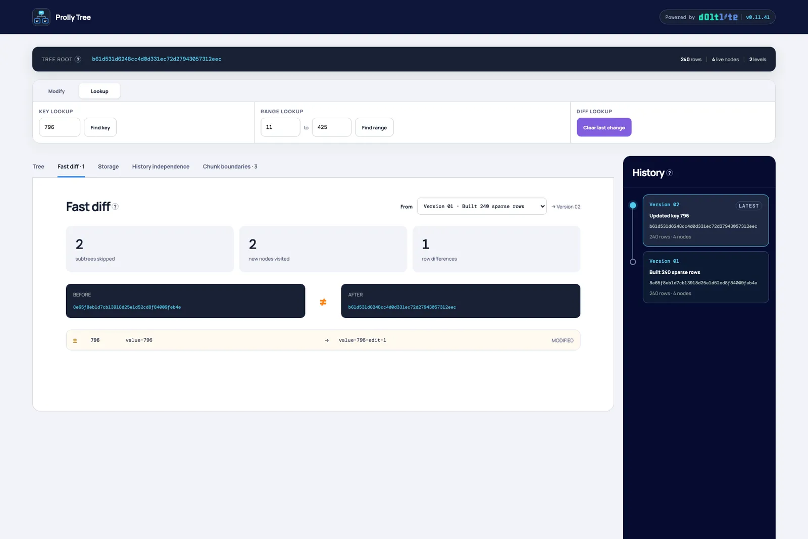
The screenshot compares the original 240-row tree with a version containing one updated value. Two subtrees are skipped, two new nodes are visited, and one modified row is returned. The root addresses differ, as they must, but most of the tree does not.

Storage#

Content addresses also buy structural sharing. A chunk is stored once regardless of how many tree versions reference it. The Storage tab counts every live tree in the timeline two ways: once as if every version owned a complete independent copy, and once by distinct content address.

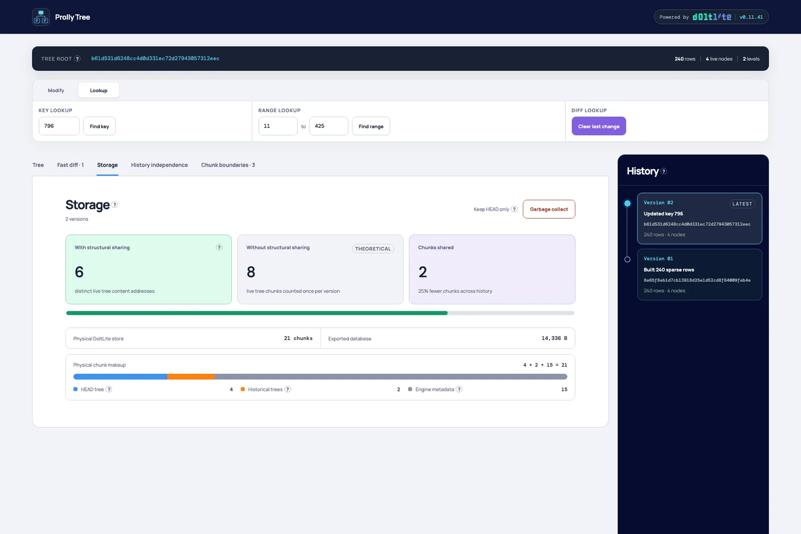
Our two versions contain four live chunks each, so storing them independently would require eight chunks. With structural sharing, the two unchanged leaves are reused and only six distinct chunks are required. That is 25% less tree storage after a single edit. As the tree and version history grow, sharing the unchanged majority matters a lot more.

The physical-store section separates the current tree, historical tree chunks, and DoltLite metadata such as the catalog, working set, refs, and commits. The numbers come from the actual exported database image, not an estimate.

The demo’s Garbage collect button throws away every intermediate version and rebuilds a fresh browser database containing only HEAD. It also verifies that the rebuilt tree has the same root address. There are no user-created Git-style commits in this visualization, so the timeline contains only disposable intermediate trees. In a real DoltLite database, commits keep their referenced history reachable.

History Independence#

History independence is the property that makes fast diff and structural sharing work across independently built trees. Given the same final key-value pairs, a Prolly Tree produces the same chunk boundaries, the same chunks, and the same root address regardless of the order used to get there.

The History independence tab puts that claim to the test using the real engine. It takes the current rows, creates a second fresh DoltLite database, inserts the rows in a deterministic shuffled order, temporarily writes draft values for some keys, and updates them to their final values along the way.

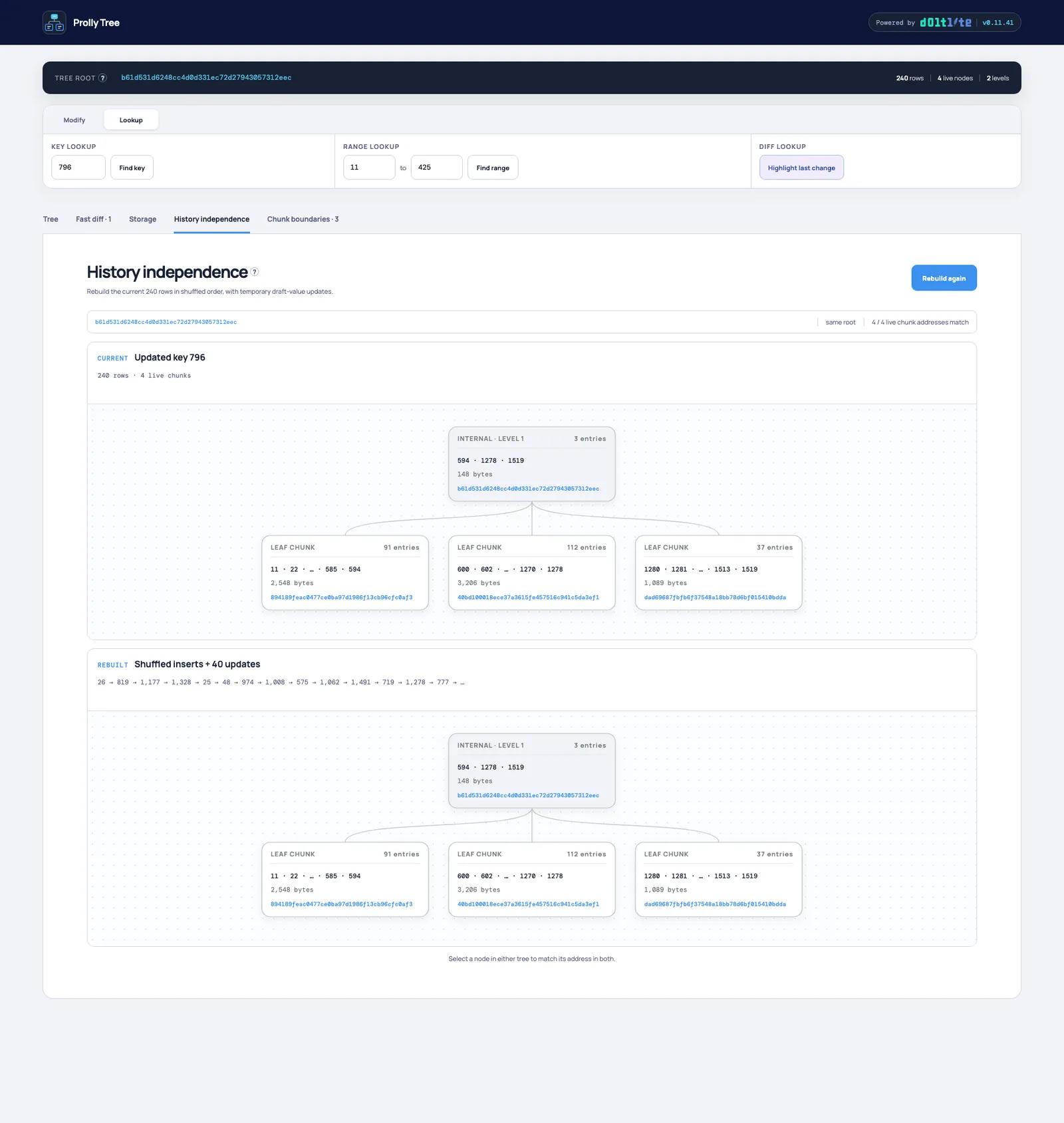
The current tree was built one way. The rebuilt tree used shuffled inserts plus 40 updates. Both finish with the same root address and the same four live chunk addresses. You can click any node in either tree and see its matching address highlighted in the other.

This is the part that still feels like magic. A B-tree’s physical shape depends on the order pages split. Two B-trees containing the same rows can look different internally. Prolly Tree boundaries are derived from the data, so two independently-built trees containing the same rows converge on the same structure. Now hash equality means something useful across history.

Chunk Boundaries#

So how are those boundaries chosen? Prolly Trees use content-defined chunking. Dolt’s implementation hashes keys and combines that deterministic result with the current chunk size to decide where a boundary falls. It targets chunks near 4KB, will not split tiny chunks, and forces a split before a chunk grows beyond its maximum size.

Despite the name “probabilistic,” the same ordered keys always produce the same boundaries. There is no runtime coin flip. Probability describes how often a key is expected to satisfy the deterministic boundary rule across different data.

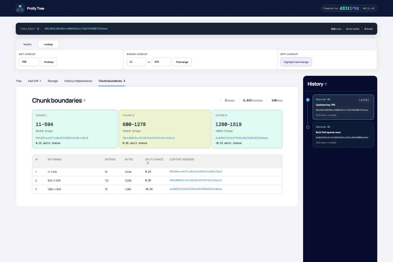
The Chunk boundaries tab lays out every live leaf with its key range, row count, encoded bytes, content address, and estimated chance that inserting an unused integer key inside that range creates a new boundary. In this example, the three chunks range from 1,089 to 3,206 bytes and the estimated split chance is less than 0.1% to 0.3%.

Splits are uncommon, but they are the expensive case. A new leaf boundary changes the parent. If the parent also crosses a boundary, the split can cascade upward. That small chance of extra work is the write tax Prolly Trees pay in exchange for fast diff, structural sharing, and history independence.

Conclusion#

I have explained Prolly Trees with thousands of words and diagrams. They are still a difficult data structure to understand. Watching a single insert rehash one path while the rest of the tree stays shared makes the whole thing click in a way a static diagram cannot.

So go play with the Prolly Tree visualizer. Insert rows. Force a split. Diff two versions. Rebuild the tree in a different order. Click everything. Once you get it, you can leverage Prolly Tree power in your own application using Dolt, Doltgres, DoltLite, or Dumbo. Every Dolt flavor is powered by this magical data structure at its core.

Find a bug or think of another property the visualizer should show? Come by our Discord and tell me. I have coding agents standing by.