Anatomy Of A SQL Engine

April 25, 2025

13 min read

May marks five years since Dolt adopted go-mysql-server. Today we summarize the current state of GMS by walking through a query's journey from parsing to result spooling.

Overview

SQL engines are the logical layer of a database that sit between client and storage. To mutate the database state on behalf of a client, a SQL engine performs the following steps:

Parsing
Binding
Plan Simplification
Join Exploration
Plan Costing
Execution
Spooling Results

Most systems also have a variety of execution strategies (row vs vector based) and infrastructure layers (run locally vs distributed). At the moment Dolt's engine by default uses row-based execution within the local server.

Parsing

The first thing a SQL Engine does when receiving a query is try to form a structured abstract syntax tree (AST). The AST is a rough cut of whether the query is well formed. The entrypoint of the parser is here.

A client driver initializes a query by passing bytes over the network through a server listener into a handler command ComHandler. The handler accumulates data until reaching a delimiter token (usually ;). The string is then split into space-delimited tokens and fed into parsing. The diagram below shows the movement from bytes to tokens and finally AST nodes:

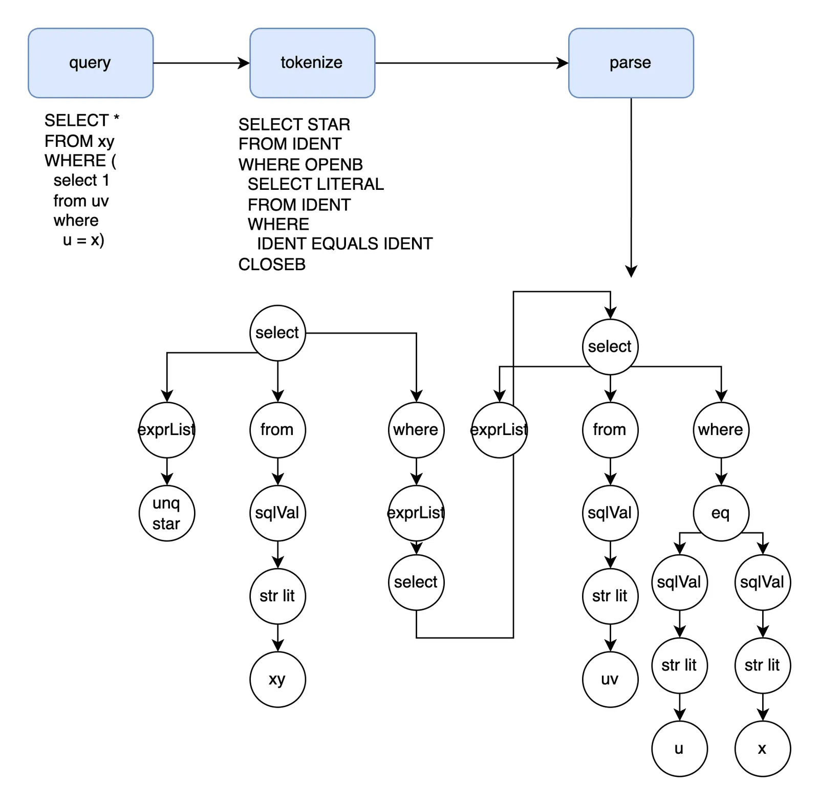
Right recursive parsing is easy to understand and debug because the program is a decision tree that chooses the next path based on the lookahead token. So a right-recursive parser might initially expect a SELECT, and then accumulate select expressions until a FROM token, and so on. This is "right recursive" because when we hit something like a join, we greedily accumulate table tokens and keep moving the parse state deeper. But right-recursive parsers are top-down, which unfortunately uses stack memory proportional to the number of tokens.

Left-recursive parsers are instead bottom-up and collapse the accumulated stack eagerly when they find a happy pattern. So when we see a join, we'll fold the join so far before checking for more tables. This keeps the memory usage low at the expense of way more complicated decision making criteria.

Dolt's Yacc grammar is left-recursive, which is fast to execute even though the shift (add token) reduce (collapse token stack) logic is hard to debug. Yacc lets us do some small formatting in stack collapse (reduce) hooks. The rules below show simplified details of what "left recursive folding" looks like from the engineer/semantic perspective:

table_reference:
  table_factor
| join_table

table_factor:
  aliased_table_name
  {
    $$ = $1.(*AliasedTableExpr)
  }
| openb table_references closeb
  {
    $$ = &ParenTableExpr{Exprs: $2.(TableExprs)}
  }
| table_function
| json_table

join_table:
  table_reference inner_join table_factor join_condition_opt
  {
    $$ = &JoinTableExpr{LeftExpr: $1.(TableExpr), Join: $2.(string), RightExpr: $3.(TableExpr), Condition: $4.(JoinCondition)}
  }

join_condition_opt:
%prec JOIN
  { $$ = JoinCondition{} }
| join_condition
  { $$ = $1.(JoinCondition) }

join_condition:
  ON expression
  { $$ = JoinCondition{On: tryCastExpr($2)} }
| USING '(' column_list ')'
  { $$ = JoinCondition{Using: $3.(Columns)} }

table_reference is the umbrella expression for the row source, either a tablescan or join. join_table is two or more tables concatenated with JOIN clauses, with the recursive table_reference portion on the left rather than the right. When the head of the stack matches join_table's definition, we pop those stack components, execute the callback hook, and replace the components with a single *JoinTableExpression on the stack. The join tree itself is right-deep, because the old state will be the left node and new state the right node in recursive calls. The unabridged version of the is here.

If parsing succeeds, the output AST is guarenteed to match the structure of our Yacc rules. If parsing fails, the client receives an error indicating which lookahead token in the query string was invalid.

Binding

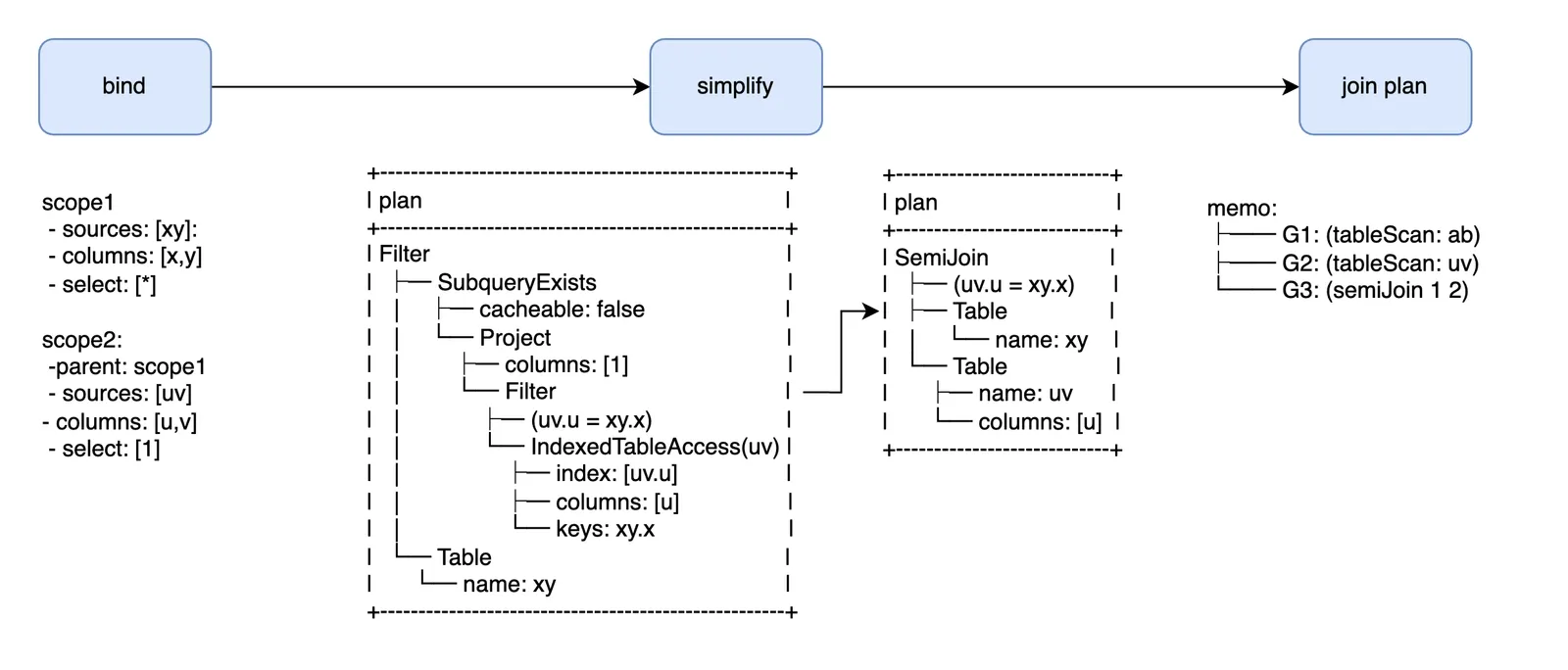
Query parsing only partially checks if a query is well formed. Fields in the AST still need to be matched to symbols in the current database catalog, in addition to a host of other typing and clause-specific checks. We call this phase "binding" because its core intermediate representation is designed for namespace scoping (code entrypoint is here).

Binding AST identifiers to catalog symbols is similar to defining and referencing variables in any programming language. Tables and aliases create column variables that column fields reference. There are ~four core objects that we can think about from a row source/sink perspective.

Table definitions are sources that provide many rows/columns. Table names cannot clash within the same scope (ex: select * from mydb.mytable.xy join xy on x), but are otherwise globally accessible. Subqueries are a special expression that add an extra namespacing layer, but otherwise act like table source: select sq.a from (select x as a from xy) sq.

Column definitions are sinks that reference a specific column from a row source. A reference in a scope with two otherwise ambiguous column names has to qualify the table to disambiguate its identity. For example, select * from xy a join xy b where x = 2 errors because the column reference in the x = 2 filter lacks a table qualifier.

Aliases are scalar sinks and sources, which is somewhat unusual. For each row in a source they output a single value. This means we add column definitions available for referencing, but only at the boundary of the original scope. For example, select x+y as a from xy where a > 2 errors because the a definition is defined and created after the filter/projection. The same query with having a > 2 is valid because HAVING has access to the second scope with the a alias.

Scalar subqueries are sources and sinks. They are similar to aliases, but with the added complexity that the subquery scopes all share the parent scope. Multiple scopes add a hierarchy to name binding, but are otherwise intuitive: search the current scope for a name match, and then iterate upwards until finding a scope with an appropriate definition. Common names cannot clash between scopes, only within. select (select a.x from xy b) from xy a is valid because even though the a.x variable is not found within the b scope, the a parent scope provides a binding.

Common Table Expressions (CTEs) and subquery aliases are simple extensions of the same namespacing rules. Aggregations have fairly specific rules about what combinations of GROUP BY and selection columns are valid, which we will not discuss here.

The binding phase converts AST nodes into customized go-mysql-server sql.Node plan nodes as outputs.

Plan Simplifications

Simplification regularizes SQL's rich syntax into a narrow format. Ideally all logically equivalent plans would funnel into one common shape. The "canonical" form should be the least surprising and fastest to execute. In practice, perfect simplification is an aspirational goal that has improved over time as workloads grow in complexity. The code entrypoint is here. The current list of rules are in this file.

Plan nodes hold correctness info calculated during binding in a format amenable to query transformations. Technically this is our third intermediate representation (IR), after ASTs and scope hierarchies. Simplifications rules are always triggered because they improve query runtime the same way compiler optimizations do dead code elimination and expression folding. Some well documented SQL simplifications are filter pushing and column pruning, which discard unused rows and columns (respectively) as soon as possible during execution.

We have dozens of simplification rules, most of which fit a narrow pattern match => rearrangement flow. The structure is so standardized that CockroachDB wrote a DSL specifically for transformations. The rules are simple and change rarely so we do it by hand, but the formalization is interesting for those who want to learn learn more.

One notable transformation that breaks the mould is subqeuery decorrelation/apply joins. A query like select * from xy where x = (select a from ab) is equivalent to select * from xy join ab on x = a. Collapsing table relations, filters, and projections into a common scope always leads to better join planning and often extra intra-scope simplifications. More formal specifications can be found here and here.

Type Coercion

The same expression's type varies depending on the calling context. For example, an expression in an insert can be cast to the target column type, while a WHERE filter expression might be cast to a boolean. Dolt's SQL engine is increasingly shifting typing from execution to binding using top-down coercion hints. Typing is usually a separate compiler phase because it shares properties of both binding and simplification. We're semantically validating the query's typing consistency and correctness, while simplifying the expressions in a way that offloads work from the execution engine.

Plan Exploration

A query plan's simplest form is often the fastest to execute. But joins, aggregations, and windows often have several equivalent variations whose performance is database dependent.

Plan exploration has two separable components, search and costing. Search enumerates valid join configurations that all produce logically equivalent results. Logical variants include order rearrangements (A x (B x C) = > (C x A) x B) and operator choice (LOOKUP_JOIN vs HASH_JOIN vs ...). Costing estimates the runtime cost of specific (physical) plan configurations.

Join Search

Within join order exploration there are two strategies. The first iteratively performs valid permutations on the seed plan, memoizing paths to avoid duplicate work. The search terminates when we run out of permutations, or decide we've found an optimal plan. The search entrypoint is here.

The top-down backtracking strategy contrasts with bottom-up dynamic programming (DP), where we instead iterate every possible join order. First we try every two-table join configuration, then every three table combo, ... etc working our way up to all n-tables.

Backtracking only visits valid states, but DP needs to detect conflicts for all combinations. For example, for A LEFT JOIN B we would invalidate any order that violates A < B. This means backtracking can miss good plans if our search doesn't reach far enough. DP invalidation criteria can be either be too broad and reject valid plans, or have holes and accidentally accept invalid plans. GMS currently uses the second strategy with a DP-Sube conflict detector that reaches more rearrangements than backtracking without sacrificing correctness.

Every valid order is expanded beyond the default INNER_JOIN plan to consider LOOKUP_JOIN, HASH_JOIN, and MERGE_JOIN, among others.

One under-appreciated point worth noting is the intermediate representation used to accumulate explored states (join orders). As a reminder, the DP subproblem optimality conditions are:

Join states can be logically clustered into groups by the results they produce.
A join group is always composed of two smaller logical join groups.

There are a variety of words used to describe this problem (hypergraph = graph of graphs, forest = tree of trees), but memo is the most common terminology we saw so we stuck with that. A memo group contains all the search states (join orders) that produce the same result, and so is identified by the bitmap AND of the node id's in the group. A specific search state is two expression groups and a physical operator, terminating it table source groups.

The initial memo for select * from join ab, uv, xy where a = u and u = x; is below:

memo:
├── G1: (tableScan: ab)
├── G2: (tableScan: uv)
├── G3: (innerJoin 2 1) (innerJoin 1 2)
├── G4: (tableScan: xy)
├── G5: (innerJoin 3 4) (innerJoin 6 1)
└── G6: (innerJoin 4 2)

Each table gets a logical expression group. Each 2-way join gets and expression group (we link a=x using the transitive property). And they all funnel into the top-level join in G5.

This organization lets us cache logical properties at the group level, the most notable of which is the lowest cost physical plan. The subproblem optimality motivating the memo happily applies to both join reordering and costing.

Functional Dependencies

Exploration can be expensive for 5+ table joins. Fortunately big joins often have star schema shaped primary key (t1 join t2 on pk1 = pk2) connections. If all join operators are connected by "strict keys", unique and non-null one to one relationships, sorting the tree by table size and connecting plans with LOOKUP_JOIN operators is often effective. The number of output rows (cardinality) is limited to the size of the first/smallest row source. Nick discuses functional dependency analysis for join planning more here. The functional dependencies code is here.

IR Intermission

Here is the the progress we've made so far since parsing the AST:

The first IR groups column definitions into scopes that help validate and bind field references. The second IR lets us perform structural optimizations on a simplified plan. And the third IR accomodates exploring join reorders in a way that facilitates our next topic, join costing.

Join Costing

Join costing identifies the fastest physical plan in every logical expression group enumerated during exploration. The coster entrypoint is here.

We have many blogs that detail join costing (collection of links here). The summary is that schemas and table key distributions affect join cost. A JOIN B might return 10 rows in one database and 10 million rows in another. A 10 row join might use a LOOKUP_JOIN to optimize for latency, while a 10 million row join might use a HASH JOIN to optimize for throughput. We represent index key distributions as histograms. Intersecting histograms roughly approximates both the count and new key distribution of the result relation. The combination of (1) input sizes, (2) result size, (3) operator choice give us (1) the IO work required to pull rows from disk, (2) in-memory overhead of operator specific data structures (ex: hash maps), and (3) the approximate CPU cycles for reading the table sources to produce the result count.

Here is what the expanded cost tree looks like for our query:

tmp2/test-branch*> select dolt_join_cost('SELECT * FROM xy WHERE EXISTS ( select 1 from uv where u = x )');
+---------------------------------------------------------------------------------------------------------------------------------------------------------------------------+
| dolt_join_cost('SELECT * FROM xy WHERE EXISTS (   select 1   from uv   where     u = x )')                                                                                |
+---------------------------------------------------------------------------------------------------------------------------------------------------------------------------+
| memo:                                                                                                                                                                     |
| ├── G1: (tablescan: xy 0.0)*                                                                                                                                              |
| ├── G2: (tablescan: uv 0.0)*                                                                                                                                              |
| ├── G3: (lookupjoin 1 2 6.6) (lookupjoin 6 1 6.6) (project: 5 0.0) (semijoin 1 2 4.0)*                                                                                    |
| ├── G4: (project: 2 0.0)*                                                                                                                                                 |
| ├── G5: (hashjoin 1 4 8.0) (hashjoin 4 1 8.0) (mergejoin 1 4 4.1) (mergejoin 4 1 4.1) (lookupjoin 1 4 6.6) (lookupjoin 4 1 6.6) (innerjoin 4 1 5.0)* (innerjoin 1 4 5.0)* |
| └── G6: (project: 2 0.0)*                                                                                                                                                 |
+---------------------------------------------------------------------------------------------------------------------------------------------------------------------------+

Each logical expression group (G)'s physical implementation options now have associated costs. For example, the first G3 implementation is a LOOKUP_JOIN between G1 and G2 that we've estimated costs 6.6 units. We differentiate between (1) the incremental work a join operator performs with (2) the accumulated cost of a choice and its dependencies. We print the incremental work rather than the accumulated work, though we might improve this function by printing both.

One note is that Dolt collects deterministic table statistics. Most databases use approximate sketches to (1) expedite refresh time, (2) minimize background work IO overhead, (3) make estimates fast, and (4) make it easier to compose higher order synthetic join estimations. Dolt's content addressable storage engine makes it somewhat easy for refreshes to only read a fraction of the database (more true for read-heavy workloads). Determinism is also fantastic for predictability. In practice, estimation overhead or higher order estimations have no performance bottlenecks for our Online Analytical Processing (OLAP) workloads.

When join costing is complete, we've discovered the optimal execution strategy.

Join Hints

The coster gives its best effort to satisfy join hints indicated after the SELECT token in a query. The docs go into more detail about hint options and use. The source code is here. Hints that are contradictory or not logically valid are usually ignored.

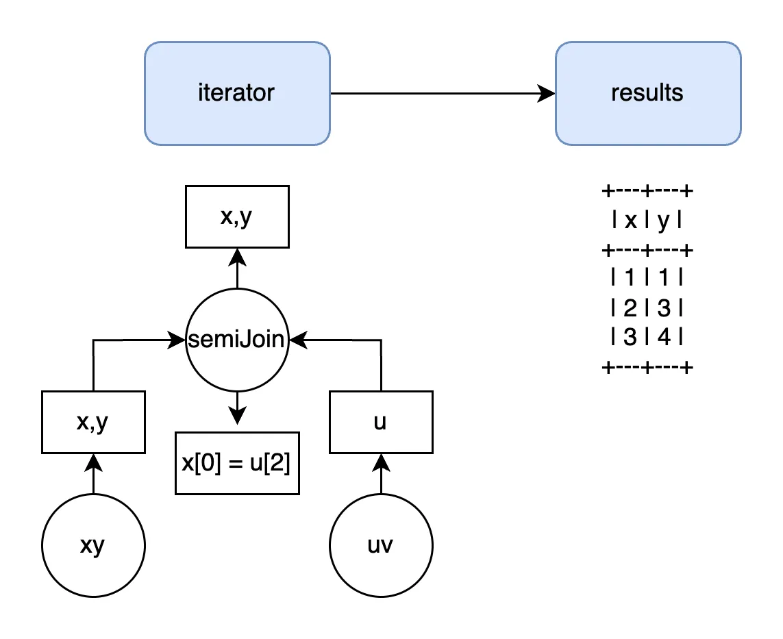
Execution

The final plan needs to be converted into an executable format.

Dolt's default row execution format mirrors the plan node format. The plan below will share a volcano iterator of the same shape:

tmp2/test-branch*> explain plan select count(*) from xy join uv on x = u;
+----------------------------------------+
| plan                                   |
+----------------------------------------+
| Project                                |
|  ├─ columns: [count(1)]                |
|  └─ GroupBy                            |
|      ├─ SelectedExprs(COUNT(1))        |
|      ├─ Grouping()                     |
|      └─ MergeJoin                      |
|          ├─ cmp: (xy.x = uv.u)         |
|          ├─ IndexedTableAccess(xy)     |
|          │   ├─ index: [xy.x]          |
|          │   ├─ filters: [{[NULL, ∞)}] |
|          │   └─ columns: [x]           |
|          └─ IndexedTableAccess(uv)     |
|              ├─ index: [uv.u]          |
|              ├─ filters: [{[NULL, ∞)}] |
|              └─ columns: [u]           |
+----------------------------------------+

Even when we swap GMS iterators with Dolt-customized kvexec iterators(example here, the abstracted iterators operating on the KV layer are still volcano iterators.

There is one notable pre-iterator conversion. The column references created in binding need to be converted from logical identifiers into offset-based index accesses. Simplification and join exploration can freely move expressions, but execution needs to know where values are located at the data layer.This analyzer rule sets the execution indexes.

Non-materializing iterators pull from the child iterator and return a row immediately. Materializing iterators have to read a sequence of children before returning. The groupByIter below shows how a GROUP_BY feeds all child rows (i.child.Next) into buffer aggregators (updateBuffers) before returning any rows (evalBuffers) (source code here):

func (i *groupByIter) Next(ctx *sql.Context) (sql.Row, error) {
	for {
		row, err := i.child.Next(ctx)
		if err != nil {
			if err == io.EOF {
				break
			}
			return nil, err
		}

		if err := updateBuffers(ctx, i.buf, row); err != nil {
			return nil, err
		}
	}

	row, err := evalBuffers(ctx, i.buf)
	if err != nil {
		return nil, err
	}
	return row, nil
}

func updateBuffers(
	ctx *sql.Context,
	buffers []sql.AggregationBuffer,
	row sql.Row,
) error {
	for _, b := range buffers {
		if err := b.Update(ctx, row); err != nil {
			return err
		}
	}
	return nil
}

func evalBuffers(
	ctx *sql.Context,
	buffers []sql.AggregationBuffer,
) (sql.Row, error) {
	var row = make(sql.Row, len(buffers))

	var err error
	for i, b := range buffers {
		row[i], err = b.Eval(ctx)
		if err != nil {
			return nil, err
		}
	}
	return row, nil
}

One wart in our execution runtime is that correlated queries are constructed dynamically at runtime. A correlated subquery is initially still represented as the plan IR during execution. The runtime prepends the scope's context to table sources in the nested query's plan before constructing a new iterator. We won't discuss the details here.

IO/Spooling

The volcano iterator in the previous stage produces result rows that need to be translated to a result format. The main code entrypoint is here.

Reading from storage and writing to network are conceptually similar even if at opposite ends of the query lifecycle. Data moves between storage, runtime, and wire-time formats the same way query plans move through different intermediate representations. Dolt's tiered storage has various real byte layouts, but we generally refer to all as the Key Value (KV) layer. Rows are represented as byte array key/value pairs in the KV layer. Any table integrator (KV layer) interfaces with GMS through in-memory arrays of Go-native types. And lastly, MySQL's wire format is completely different than either the KV or SQL formats! Integers, for example, are represented as strings in wire format.

Batching and buffer reuse help manage throughput and memory churn at each of these interfaces. Cutting out the middleman and converting from KV->wire layer is an effective optimization for many queries. Queries that return one row are common, and have specialized spooling interfaces that optimize for latency rather than throughput.

The client protocol collects result bytes until the terminal packet is sent, termination the command and freeing the session to start another query.

Future

AST are a great intermediate representation for organizing tokenized bytes, but lack the expressivity required for the rest of semantic validation, plan simplification, and join planning. Building additinal IRs for each phase created an organizational and performance problem that only unifying solves. We've redistributed most logic on SQL nodes into either the preceding (binding) or following (memo) phases. But closing the gap is still quite a lift, and could involve (1) rewriting all subquery expressions as lateral joins, and (2) representing aliases as SyntheticProject nodes that append one column definition to the tree.

Golang's automatic memory management helped us get a fully functioning database off the ground quickly, but memory churn is still a bottleneck. We have improved memory re-use at specific points in the execution lifecycle where memory is short-lived, for example spooling rows over the network, but there is still much more to do. Avoiding heap allocating interface types and reusing execution buffers would improve execution performance. Standardizing and centralizing the memo IR would probably let us reuse memory there as well.

If you have any questions about Dolt, databases, or Golang performance reach out to us on Twitter, Discord, and GitHub!

Blog